Twin Cities Marathon Data Analysis
For my Data Analysis & Visualization course this fall in my Master of Marketing Analytics program, I analyzed geographical trends in the results from the Twin Cities Marathon from the years 2015-2019.
In total, this came out to about 38,000 rows of data, on which I performed logistic regressions for runner’s home state, the number of times a runner ran the race (with some caveats), and year of participation, in order to understand trends in completion time.
- Introduction
- High-Level Findings: What factors predict a fast race time?
- Visualizations
- How Many Unique Participants?
- Appendix: Regressions
Introduction
I wanted to take a look at some historical data from the Twin Cities Marathon. I collected this data by navigating to the event results. MTEC stores event results over many years (in this case, from 2001-2019), so I was able to get the event results without too much difficulty.
Data Manipulation
However, the data isn’t returned by an end-user accessible API call, so I wound up retrieving the data manually, 500 results at a time, copying each page’s results into a file, which I saved as .tsv, then converted to .csv using Excel.
Additionally, there were some more pieces of information I wanted: I wanted to be able to use this data in the future without worrying about accidentally releasing a CSV of people’s names and hometowns and ages (just because MTEC does it doesn’t mean I should), so I wrote a Python script to hash the names.
In this script, I also retrieved latitude and longitude for the provided hometown of each participant as well as “distance from start line” (which was really just approximate miles to Minneapolis, where the race starts).
Technically, Mapbox, which was my geocoding provider, limits you to 600 requests per minute. I wasn’t 100% sure whether any requests that were rate-limited would be counted toward my monthly use. You get 100,000 free requests per month and I have about 38,000 rows, so I only really wanted to have to run this on my complete dataset once.
For those reasons, I added a timer that would wait if we had hit out minute limit on requests (the limit was 600, so I stopped at 599 because frankly I think it’s best not to tempt fate).
I then used geopy against the geocoded latitude/longitude to retrieve distance to the start line. I preserved latitude and longitude even though, at the time, I thought I only wanted to use distance to the start line, and I’m glad I did because that let me map the data, which was much easier to think about than aggregates like mean distance.
High-Level Findings: What factors predict a fast race time?
What factors are a good predictor of race time? To solve this, I ran several logistic regressions!
Does state influence race times?
Does the number of times you’ve run TCM between 2015-2019 influence probability of running the race in under 3:30?
I intend to one day run a marathon in under 3:30, and when I ran the Twin Cities Marathon, so I wanted to understand what factors are correlated with running the race under that amount of time.
Times Run vs State vs Sex
First, I ran a regression for Hours under 3:30 against the number of times run (as an integer) and state (as dummy-coded values) - (see regression 1 in appendix)
- The significant factors (P ≤ 0.1) in this regression were:
- Times you’re run this race between 2015-2019
- slightly positively correlated with strong significance
- Being from the following states/territories:
- Colorado:
- Positively correlated (0.563433), very strong significance
- Washington, D.C:
- Positively correlated (0.591973) with significance
- Minnesota:
- Negatively correlated (-0.449123) with very strong significance
- New Mexico:
- Positively correlated (1.969353) with very strong significance
- Ontario:
- Positively correlated (0.413816) with “weak” (but still statistically significant) significance (0.087 < .1)
- Oregon:
- Positively correlated (0.60625) with significance
- Washington:
- Positively correlated (0.699211) with strong significance
- Colorado:
- Being (registering for the race as) female:
- Negatively correlated (-2.069862) with “weak” significance
- Times you’re run this race between 2015-2019
The results that stand out here are the “very strong” significances - runners from Colorado, New Mexico, and Washington run faster, and runners from Minnesota run slower.
Are these results surprising? Not especially.
The lowest P value is New Mexico’s (2.63e-11) and it has the highest coefficient as well - I looked at the first 20 men to finish the race each of the five years and seventeen of those 100 total results were out of New Mexico. New Mexico is at elevation and is hot in the summer, both of which lend themselves well to racing fast in Minnesota’s cold October weather at low elevation (Minneapolis/St. Paul have similar elevations to Austin). New Mexico’s reputation as a training hotbed is well-documented.
Colorado is similarly unsurprising - Boulder is a training hotbed as well, with multiple pro teams forming training camps there in the past few years. They have high elevation, lots of summer sun, and hard winters, which build mental toughness, so it’s a great place to train whether you’re a pro or an amateur like me.
Minnesota’s negative correlation makes sense in the context of the popularity of the race among locals. More locals of all times would likely bring their results closer to the mean time (just under 4:30).
Times Run as an Integer or Factor
Next, I ran a regression for Hours under 3:30 against the number of times run (as dummy-coded values) (Regression 2) and number of times ran as an integer (Regression 3) to compare results
In the integer regression, times you’ve run the race is somewhat positively correlated (0.09113) with strong statistical significance (P=2.26e-14, wow!!)
In the dummy coded regression, times you’ve run the race is positively correlated at every statistically significant factor (2, 3, 4, 5 and 10 times) with 10 being weakly significant.
This analysis requires some context on what I’ve called the common name effect, discussed below to find that discussion quickly, but in short, the analyses over 5 should be ignored because they are the effect of a participant sharing a name with another participant within or between years.
Year of Participation
Finally, I did a regression to analyze against the year of participation and number of times run as factors (Regression 4), and just the year of participation (Regression 5):
The coefficients for number of times run changed and running the race 5 times became more strongly significant, but no factors were significant in this regression that weren’t in the previous.
The base case in this regression was 2015 with a participant who only ran the race once. Every other year had a negative, coefficient (so, you’re more likely to run under 3:30 in 2015 than any other year). However, only 2017 was statistically significant (and it was very strongly significant with P=1.18e-05) - it had a coefficient of -0.217072. To understand this better, I looked at weather on those two days: in 2017 it was 55 degrees Fahrenheit at 8AM whereas in 2015 it was 42 and didn’t hit 55 until noon (at noon in 2017 it was 60).
Finally, in the year-only regression (Regression 5) - again, only the intercept and 2017 are statistically significant, but this time, 2016, 2016, and 2019 are negatively correlated and 2018 is positively (and not statistically significantly) correlated.
Visualizations
# install.packages("dplyr")    # alternative installation of the %>%
library(dplyr)    # alternatively, this also loads %>%
library("ggplot2")


# install.packages("maps")
library(maps)     # Provides latitude and longitude data for various maps

included_years<-c(2015,2016,2017,2018,2019)
library(lubridate)
# String manipulation
library(stringr)

# Verbose regular expressions
library(rebus)

library(aod)to_seconds<- function(time_element){
seconds<-0
time_arr <- strsplit(time_element, ':')
length(time_arr)
for (i in 1:length(time_arr[[1]])){
factor <- 3 - i
seconds <- seconds + ((60^factor) * strtoi(time_arr[[1]][i], base=10))
}
return(seconds)
}
tcm<-read.csv('./anonymized_tcm_2019.csv')
tcm_2018<-read.csv('./anonymized_tcm_2018.csv')
tcm_2017<-read.csv('./anonymized_tcm_2017.csv')
tcm_2016<-read.csv('./anonymized_tcm_2016.csv')
tcm_2015<-read.csv('./anonymized_tcm_2015.csv')
sponsors <- read.csv('./Sponsors.csv')
us_states <- read.csv('./states.csv')tcm_2019 <- tcm%>%rowwise()%>%mutate(seconds = to_seconds(Time))
tcm_2018 <- tcm_2018%>%rowwise()%>%mutate(seconds = to_seconds(Time))
to_seconds(tcm_2018$Time)## [1] 7918tcm_2017 <- tcm_2017%>%rowwise()%>%mutate(seconds = to_seconds(Time))
tcm_2016 <- tcm_2016%>%rowwise()%>%mutate(seconds = to_seconds(Time))
tcm_2015 <- tcm_2015%>%rowwise()%>%mutate(seconds = to_seconds(Time))
tcm_2019 <- tcm_2019%>%rowwise()%>%mutate(Year = 2019)%>%mutate(YearsSince2015 = 2019-2015)
tcm_2018 <- tcm_2018%>%rowwise()%>%mutate(Year = 2018)%>%mutate(YearsSince2015 = 2018-2015)
tcm_2017 <- tcm_2017%>%rowwise()%>%mutate(Year = 2017)%>%mutate(YearsSince2015 = 2017-2015)
tcm_2016 <- tcm_2016%>%rowwise()%>%mutate(Year = 2016)%>%mutate(YearsSince2015 = 2016-2015)
tcm_2015 <- tcm_2015%>%rowwise()%>%mutate(Year = 2015)%>%mutate(YearsSince2015 = 2015-2015)
all_tcms <- rbind(tcm_2019, tcm_2018, tcm_2017, tcm_2016, tcm_2015)
seconds_in_an_hour<-60.0*60.0
all_tcms <- all_tcms%>%rowwise()%>%
mutate(Lat = gsub( "\\[", "",strsplit(LatLong,", " )[[1]][1])[[1]][1] )%>%
mutate(Long = gsub( "\\]", "",strsplit(LatLong,", " )[[1]][2])[[1]][1])%>%
mutate(inMinn=State=="MN")%>%
mutate(Hours=as.double(seconds)/seconds_in_an_hour)Changing Participation Rates
Participation decreased since 2015:
head(all_tcms)## # A tibble: 6 x 19
## # Rowwise:
## Bib Name Sex Age City State Overall SexPl DivPl Time LatLong
## <int> <chr> <chr> <chr> <chr> <chr> <chr> <chr> <chr> <chr> <chr>
## 1 2 75f5… M 31 Sant… NM Jan-47 Jan-… 1 / … 2:12… [35.68…
## 2 8 2279… M 29 Colo… CO Feb-47 Feb-… 1 / … 2:13… [38.83…
## 3 4 bf90… M 29 Minn… MN Mar-47 Mar-… 2 / … 2:15… [44.97…
## 4 35 3771… M 25 Gosh… CT Apr-47 Apr-… 3 / … 2:16… [41.83…
## 5 10 362f… M 24 Port… OR May-47 May-… 1 / … 2:17… [45.52…
## 6 11 ca63… M 27 Sout… UT Jun-47 Jun-… 4 / … 2:18… [40.70…
## # … with 8 more variables: DistanceToStartLine <dbl>, seconds <dbl>,
## # Year <dbl>, YearsSince2015 <dbl>, Lat <chr>, Long <chr>, inMinn <lgl>,
## # Hours <dbl>count_by_year_aggregate <-all_tcms %>% group_by(Year)
participation_years<-all_tcms%>%count(YearsSince2015)
sponsor_years<-sponsors%>%count(YearsSince2015)
print(participation_years)## # A tibble: 5 x 2
## # Rowwise:
## YearsSince2015 n
## <dbl> <int>
## 1 0 8546
## 2 1 8561
## 3 2 7490
## 4 3 7144
## 5 4 6747ggplot(data=all_tcms) + geom_histogram(aes(x=YearsSince2015) )+ labs(title="Race sizes by year")
pcp_line<-coef(lm(participation_years$n ~ participation_years$YearsSince2015))

ggplot(data=participation_years, aes(x=YearsSince2015, y=n)) + geom_point( )+ labs(title="Participation/Year") +geom_smooth(method = "lm", se = FALSE) +
geom_abline(intercept = pcp_line["(Intercept)"], slope = pcp_line["participation_years$YearsSince2015"]) + geom_text(
  aes(label=round(..y.., 2), y = n, x=YearsSince2015),stat = 'summary',
  nudge_y = 100,
  va = 'bottom', fun.y="mean"
)
print(pcp_line)## (Intercept) participation_years$YearsSince2015
## 8700.6 -501.5Chicago Marathon Effect (maybe)
The Twin Cities Marathon and the Chicago Marathon are both held in early October, so it’s worth considering whether holding the events in different weekends would lead to increased participation.
tcm_chicago<-read.csv("./tcm_chicago_dates.csv")
tcm_chicago<-tcm_chicago%>%full_join(all_tcms%>%count(Year), by="Year")
tcm_chicago<-tcm_chicago%>%mutate(TCM_days_before_Chicago = time_length(as.Date(as.character(tcm_chicago$TCM.Date), format="%m/%d/%Y")-
                  as.Date(as.character(tcm_chicago$Chicago.Date), format="%m/%d/%Y"), unit="days"))
tcm_chicago<-tcm_chicago%>%mutate(less_participants_than_previous_year = time_length(as.Date(as.character(tcm_chicago$TCM.Date), format="%m/%d/%Y")-
                  as.Date(as.character(tcm_chicago$Chicago.Date), format="%m/%d/%Y"), unit="days"))
ggplot(data=tcm_chicago, aes(x=Year, y=n, fill=TCM_days_before_Chicago )) + geom_bar(stat = "summary", fun.y = "mean" )+ labs(title="Participation/Year") 
I don’t have a decade’s worth of data, so I can’t say something conclusive either way, however this doesn’t look meaningful. This makes sense considering what a large percentage of participants are from Minnesota and likely run this race out of convenience or love of their hometown or state. Their pull to the race is likely explained by something other than a love of road racing.
A Side Note: Effect of Sponsorship
Let’s look at sponsor data:
I got the sponsor data by browsing the Internet Archive and manually compiling each page’s results into a CSV including sponsor name, year, and sponsorship level.
# https://web.archive.org/web/20150905060407/https://www.tcmevents.org/sponsors/
# https://web.archive.org/web/20160820100234/https://www.tcmevents.org/sponsors/
# https://www.tcmevents.org/sites/default/files/2017-09/2017%20Medtronic%20Twin%20Cities%20Marathon%20Participant%20Guide%20final.pdf
# https://www.tcmevents.org/sites/default/files/2018-09/2018%20Marathon%20Participant%20Guide.pdf
# https://www.tcmevents.org/events/medtronic-twin-cities-marathon-weekend-2019/race/marathon


ggplot(data=all_tcms) + geom_histogram(aes(x=Year) )+ labs(title="Race sizes by year")
ggplot(data=sponsors) + geom_histogram(aes(x=Year) )+ labs(title="Number of sponsors by year")
If I had more years of data readily accessible, I would investigate how the number of sponsors in a year impacts the rate of participation that year or in subsequent years.
Are Finish Times Slowing Down?
Let’s look at some summary statistics:
In short, not really. This is most likely largely explainable by weather.
summary(all_tcms)## Bib Name Sex Age
## Min. : 1 Length:38488 Length:38488 Length:38488
## 1st Qu.: 3392 Class :character Class :character Class :character
## Median : 6004 Mode :character Mode :character Mode :character
## Mean : 6221
## 3rd Qu.: 9024
## Max. :12775
##
## City State Overall SexPl
## Length:38488 Length:38488 Length:38488 Length:38488
## Class :character Class :character Class :character Class :character
## Mode :character Mode :character Mode :character Mode :character
##
##
##
##
## DivPl Time LatLong DistanceToStartLine
## Length:38488 Length:38488 Length:38488 Min. : 0.000
## Class :character Class :character Class :character 1st Qu.: 8.252
## Mode :character Mode :character Mode :character Median : 17.810
## Mean : 260.423
## 3rd Qu.: 233.722
## Max. :10636.434
## NA's :10
## seconds Year YearsSince2015 Lat
## Min. : 7731 Min. :2015 Min. :0.00 Length:38488
## 1st Qu.:13773 1st Qu.:2016 1st Qu.:1.00 Class :character
## Median :15560 Median :2017 Median :2.00 Mode :character
## Mean :15701 Mean :2017 Mean :1.87
## 3rd Qu.:17546 3rd Qu.:2018 3rd Qu.:3.00
## Max. :22891 Max. :2019 Max. :4.00
##
## Long inMinn Hours
## Length:38488 Mode :logical Min. :2.147
## Class :character FALSE:12069 1st Qu.:3.826
## Mode :character TRUE :26419 Median :4.322
## Mean :4.362
## 3rd Qu.:4.874
## Max. :6.359
## ggplot(data=all_tcms) + geom_bar(aes(y=seconds, x=Year), stat="summary", fun.y="mean" )+ labs(title="Race pace by year") + geom_text(
aes(label=round(..y.., 2), y = seconds, x=Year),
stat = 'summary',
nudge_y = 10,
va = 'bottom', fun.y="mean"
)
How far are participants from the start line?
Minnesotans love this race:
ggplot(data=all_tcms) + geom_histogram(aes(x=DistanceToStartLine) , bins=200)+ labs(title="Average distance to start line")
More Minnesotans in Minneapolis/St. Paul participated than those outside the metro.
ggplot(data=all_tcms%>%filter(State=="MN")) + geom_histogram(aes(x=DistanceToStartLine) , bins=200)+ labs(title="Average distance to start line, Minnesotans")
And, unsurprisingly, there are more non-Minnesotans who are closer to the start line who run this race than Minnesotans who are far:
ggplot(data=all_tcms%>%filter(State!="MN")) + geom_histogram(aes(x=DistanceToStartLine) , bins=200)+ labs(title="Average distance to start line, non-Minnesotans")
By Distance
ggplot(data=all_tcms %>%rowwise()%>%
    filter(DistanceToStartLine>10.0)) + geom_histogram(aes(x=DistanceToStartLine) , bins=100)+ labs(title="Distance to start line",subtitle="participants over 20 mi away")
ggplot(data=all_tcms %>%rowwise()%>%
    filter(DistanceToStartLine>50.0)) + geom_histogram(aes(x=DistanceToStartLine) , bins=100)+ labs(title="Distance to start line",subtitle="participants over 50 mi away")
ggplot(data=all_tcms %>%rowwise()%>%
    filter(DistanceToStartLine>200.0)) + geom_histogram(aes(x=DistanceToStartLine) , bins=100)+ labs(title="Distance to start line",subtitle="participants over 200 mi away")
ggplot(data=all_tcms %>%rowwise()%>%
    filter(DistanceToStartLine>1000.0)) + geom_histogram(aes(x=DistanceToStartLine) , bins=100)+ labs(title="Distance to start line",subtitle="participants over 1000 mi away")
Participants out of Minnesota
library(usmap)
library(maptools)
library(rgdal)
I wanted to do some visualizations of this data, but the overwhelming amount of participants from Minnesota makes it hard to look at, frankly, so I split Minnesota out of the results:
pcp_locations<- all_tcms%>%filter(State %in% us_states$Abbreviation)%>%filter(! is.na(State))%>%select(Long, Lat, seconds, State, Year)%>%mutate(Long=as.numeric(Long), Lat=as.numeric(Lat))%>%mutate(Hours=seconds%/%(60*60))

out_of_us_locations<- all_tcms%>%filter(!State %in% us_states$Abbreviation)%>%filter(! is.na(State))%>%select(Long, Lat, seconds, State)%>%mutate(Long=as.numeric(Long), Lat=as.numeric(Lat))%>%mutate(Hours=seconds%/%(60*60))

pcp_locations <- na.omit(pcp_locations)

out_of_us_locations<-na.omit(out_of_us_locations)

eq_transformed <- usmap_transform(pcp_locations)

eq_transformed<-eq_transformed%>%filter(Lat.1>=-4000000)%>%filter(Lat.1<=2000000)%>%filter(Long.1>=-2500000)%>%filter(Long.1<=2000000)

eq_mn<-eq_transformed%>%filter(State=="MN")
eq_not_mn<-eq_transformed%>%filter(State!="MN")
eq_transformed_2 <- usmap_transform(out_of_us_locations)

plot_usmap() +
  geom_point(data = eq_mn, aes(x = Long.1, y = Lat.1),
             color = "red", alpha = 0.1, size=0.1) +
             geom_point(data = eq_not_mn, aes(x = Long.1, y = Lat.1),
             color = "blue", alpha = 0.1, size=0.1) +

  labs(title = "Marathon Finishers, In & Out of Minnesota") +
  theme(legend.position = "right")
And I removed them altogether to look at non-Minnesotan participant density by state:
out_of_state_density<-pcp_locations%>%filter(State!="MN")%>%count(Year, State)%>%mutate(state=State)

plot_usmap(data = out_of_state_density, values="n") +
scale_fill_continuous( high = "#4c476a", low = "white",
                         name = "Participants", label = scales::comma
  ) +

  labs(title = "Marathon Finisher Density Outside of Minnesota") +
  theme(legend.position = "right")+facet_wrap(~Year)
out_of_state_times<-pcp_locations%>%filter(State!="MN")

out_of_state_times<-aggregate(Hours~State, data=out_of_state_times, FUN=mean)%>%mutate(state=State)


plot_usmap(regions = "state",data = out_of_state_times, values="Hours") +
scale_fill_continuous( high = "#4c476a", low = "white",
                         name = "Participant Times (Hours)", label = scales::comma) +

  labs(title = "Marathon Finisher Times Outside of Minnesota") +
  theme(legend.position = "right")
pcp_aggr<- all_tcms%>%group_by(State, Year)%>%mutate(Abbreviation=State)%>%filter(State %in% us_states)

gusa <- left_join(map_data("state"), us_states%>%mutate(region=tolower(State)), "region")

gusa_pcps <- left_join(gusa, pcp_aggr, "Abbreviation")

states_by_aggr<-select(pcp_aggr, region=State)
How Many Unique Participants?
We have 38488 unique records - Interestingly enough, we have 29504 unique participant names and only 3279 unique participant locations:
nrow(all_tcms)## [1] 38488sapply(all_tcms, function(x) length(unique(x)))## Bib Name Sex Age
## 11825 29504 3 77
## City State Overall SexPl
## 3001 84 38488 34629
## DivPl Time LatLong DistanceToStartLine
## 35823 10839 3279 3279
## seconds Year YearsSince2015 Lat
## 10839 5 5 3225
## Long inMinn Hours
## 3245 2 10839Results For One-Time Participants
Disclaimer
When doing this analysis, I wanted to look at the differences between participants who had run this event once in the five years and participants who ran the event multiple times in the five years. Of course, the problem with this approach was that some participants will run the event once but have very common names (i.e. the John Smiths of the world) and it isn’t farfetched to expect at least one participant will run the event more than once but change their name between participations (i.e. Beyoncé Knowles and Beyoncé Knowles-Carter).
I originally assumed the data would be completely unusable for this reason - surely there are a large number of participants with the same name running in the same or different years.
To validate my concerns, I looked at the 2019 results on the MTEC website, and what I found surprised me a bit:

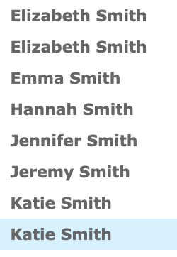
I looked at the most common surnames in Minnesota (because, as we’ve seen, most participants are from Minnesota and Minnesota’s ethnic makeup is very different than that of my home state, Texas), to make sure I wasn’t overlooking something that should be obvious.
It looks like the top chances of repeat names are:
- Johnson
- Anderson
- Nelson
- Olson
- Peterson
- Smith
- Larson
- Miller
Between those surnames for 2019, I only found one instance of triple names and a few double instances (which appeared to increase based on name commonness in and outside of Minnesota, so, more doubles for Andersons and Millers than Larsons).
Based on this soft analysis and the size of the race, I’m less worried about common names messing up the broad trends of this data.
For a larger race such as the Chicago Marathon or for an analysis using more years, I would be much more worried about this effect and how it compounds over the years.
For the remainder of this analysis, I will call this the Common Name Effect
Cleaning the Analysis
When replicating this research for another race where the same columns are provided, I will consider these steps to get a more clean analysis (these are ranked based on ease of implementation):
- Create a column combining hashed name, city, and state and group for uniqueness on that column
- Create a column for approximate year of birth based on age at time of racing and the year of the race and group for uniqueness on that column
The second method is better because people can and do move, but worse because repeat participants born in early October could be counted as unique participants based on whether the race is before or after their birthday that year.
The Results
Note that I am removing participants who appear in this data more than 5 times, because it has clearly been affected by the common name effect.
grouped_by_name<-all_tcms%>%group_by(Name)%>%mutate(times_run=as.integer(n()))

repeats<-grouped_by_name%>%filter(n()>1)%>%filter(n()<6)
nrow(repeats)
## [1] 14390ggplot(data=repeats) + geom_bar(aes(x=times_run, y=Hours, fill=Year),stat = "summary", fun.y = "mean", position="dodge" ) + labs(title="Mean Finishing Time, Repeat Participants")
ggplot(data=repeats%>%ungroup()) + geom_bar(aes(x=times_run, y=Hours, fill=Year),stat = "summary", fun.y = "mean", position="dodge" ) + labs(title="Mean Finishing Time, Repeat Participants")
onesies<-grouped_by_name%>%filter(n()==1)Geography For One-Timers
out_of_state_density<-onesies%>%ungroup()%>%filter(State %in% us_states$Abbreviation)%>%filter(! is.na(State))%>%select(Long, Lat, seconds, State, Year)%>%mutate(Long=as.numeric(Long), Lat=as.numeric(Lat))

map_density<-out_of_state_density%>%count(Year, State)%>%mutate(state=State)


plot_usmap(data = map_density%>%filter(State!="MN"), values="n") +
scale_fill_continuous( high = "#4c476a", low = "white",
                         name = "Participants", label = scales::comma
  ) +
  labs(title = "One Time Twin Cities Marathon Participants Density, Minnesota Removed, All Years") +
  theme(legend.position = "right")
plot_usmap(data = map_density%>%filter(State!="MN"), values="n") +
scale_fill_continuous( high = "#4c476a", low = "white",
                         name = "Participants", label = scales::comma
  ) +
  labs(title = "One Time Twin Cities Marathon Participants Density, Minnesota Removed") +
  theme(legend.position = "right")+facet_wrap(~Year)
in_state_density<-repeats%>%ungroup()%>%filter(State %in% us_states$Abbreviation)%>%filter(! is.na(State))%>%select(Long, Lat, seconds, State, Year)%>%mutate(Long=as.numeric(Long), Lat=as.numeric(Lat))

map_density<-in_state_density%>%count(Year, State)%>%mutate(state=State)

plot_usmap(data = map_density%>%filter(State!="MN"), values="n") +
scale_fill_continuous( high = "#4c476a", low = "white",
                         name = "Participants", label = scales::comma
  ) +
  labs(title = "Repeat Twin Cities Marathon Participants Density, Minnesota Removed, All Years") +
  theme(legend.position = "right")
plot_usmap(data = map_density%>%filter(State!="MN"), values="n") +
scale_fill_continuous( high = "#4c476a", low = "white",
                         name = "Participants", label = scales::comma
  ) +
  labs(title = "Repeat Twin Cities Marathon Participants Density, Minnesota Removed") +
  theme(legend.position = "right")+facet_wrap(~Year)
Appendix: Regressions
Regression 1: States
ungrouped_for_logit<-grouped_by_name%>%ungroup()%>%mutate(sub_three_thirty=as.integer(as.logical(Hours<=3.5)),sub_five=as.integer(as.logical(Hours<=5.0)))

ungrouped_for_logit$State <- factor(ungrouped_for_logit$State)
ungrouped_for_logit$Sex <- factor(ungrouped_for_logit$Sex)
ungrouped_for_logit$Minnesotan <- factor(ungrouped_for_logit$inMinn)

mylogit_state <- glm(sub_three_thirty ~ times_run + State+Sex, data = ungrouped_for_logit, family = "binomial")

summary(mylogit_state)
##
## Call:
## glm(formula = sub_three_thirty ~ times_run + State + Sex, family = "binomial",
## data = ungrouped_for_logit)
##
## Deviance Residuals:
## Min 1Q Median 3Q Max
## -1.4823 -0.5797 -0.3872 -0.2932 2.5174
##
## Coefficients:
## Estimate Std. Error z value Pr(>|z|)
## (Intercept) -0.684752 1.244444 -0.550 0.582150
## times_run 0.078090 0.012476 6.259 3.87e-10 ***
## StateAA -13.238809 882.743385 -0.015 0.988034
## StateAB 0.863555 0.604664 1.428 0.153247
## StateAE -12.917519 497.796832 -0.026 0.979298
## StateAK 0.422212 0.435463 0.970 0.332261
## StateAL 0.227157 0.522677 0.435 0.663851
## StateAR -0.121597 0.466754 -0.261 0.794465
## StateAZ 0.008583 0.333578 0.026 0.979472
## StateB. -13.238809 882.743386 -0.015 0.988034
## StateBC -12.638823 284.137288 -0.044 0.964521
## StateBU -13.238809 882.743384 -0.015 0.988034
## StateCA 0.272634 0.176225 1.547 0.121844
## StateCAN -13.238809 882.743384 -0.015 0.988034
## StateCD 2.020406 1.231657 1.640 0.100923
## StateCO 0.563433 0.169985 3.315 0.000918 ***
## StateCT 0.474084 0.326304 1.453 0.146255
## StateDC 0.591973 0.295371 2.004 0.045052 *
## StateDE -0.059035 1.125601 -0.052 0.958172
## StateDF -13.238809 882.743385 -0.015 0.988034
## StateDI -13.238809 882.743384 -0.015 0.988034
## StateFL -0.369913 0.238805 -1.549 0.121378
## StateGA -0.332890 0.273754 -1.216 0.223978
## StateGE -13.238809 882.743385 -0.015 0.988034
## StateGU 0.235954 0.816673 0.289 0.772642
## StateHE 15.893327 882.743385 0.018 0.985635
## StateHI -13.015892 305.340219 -0.043 0.965998
## StateIA 0.001918 0.159655 0.012 0.990413
## StateIB -13.238809 882.743384 -0.015 0.988034
## StateID -0.378136 0.555472 -0.681 0.496031
## StateIL -0.230399 0.160465 -1.436 0.151054
## StateIN 0.170085 0.272073 0.625 0.531876
## StateJA -12.488142 347.980878 -0.036 0.971372
## StateKA -13.238809 882.743385 -0.015 0.988034
## StateKEN 15.659057 882.743385 0.018 0.985847
## StateKS 0.118278 0.261775 0.452 0.651390
## StateKY -0.230849 0.462892 -0.499 0.617983
## StateLA 0.057413 0.563359 0.102 0.918827
## StateM -13.238809 882.743385 -0.015 0.988034
## StateMA 0.335102 0.208783 1.605 0.108489
## StateMB 0.100101 0.213878 0.468 0.639766
## StateMD -0.041499 0.291019 -0.143 0.886606
## StateME 0.712600 0.467940 1.523 0.127797
## StateMI 0.041947 0.204046 0.206 0.837120
## StateMN -0.449123 0.132243 -3.396 0.000683 ***
## StateMO 0.141741 0.221131 0.641 0.521533
## StateMS -0.505038 0.768666 -0.657 0.511161
## StateMT 0.201664 0.393923 0.512 0.608695
## StateNC 0.127820 0.255465 0.500 0.616834
## StateND -0.014092 0.194425 -0.072 0.942220
## StateNE 0.131102 0.226096 0.580 0.562014
## StateNH -0.111335 0.567744 -0.196 0.844531
## StateNJ 0.447851 0.285989 1.566 0.117355
## StateNM 1.969353 0.295443 6.666 2.63e-11 ***
## StateNO 2.001892 1.501145 1.334 0.182343
## StateNS -12.000807 508.623331 -0.024 0.981176
## StateNU 1.476197 1.293017 1.142 0.253592
## StateNV 0.366756 0.688393 0.533 0.594191
## StateNY 0.220708 0.192746 1.145 0.252179
## StateOH 0.118531 0.242865 0.488 0.625514
## StateOK -0.008182 0.390503 -0.021 0.983283
## StateON 0.413816 0.241857 1.711 0.087082 .
## StateOR 0.606250 0.295794 2.050 0.040406 *
## StatePA -0.051262 0.248933 -0.206 0.836848
## StatePU -13.316899 882.743385 -0.015 0.987964
## StateQC 0.289890 0.825047 0.351 0.725318
## StateRI 0.788655 1.207591 0.653 0.513704
## StateSA -12.580380 381.039232 -0.033 0.973662
## StateSC 0.497764 0.458153 1.086 0.277277
## StateSD 0.037688 0.205420 0.183 0.854431
## StateSK -12.708897 426.740273 -0.030 0.976241
## StateSP -13.238809 882.743385 -0.015 0.988034
## StateTE -11.889543 882.743386 -0.013 0.989254
## StateTN 0.102227 0.343045 0.298 0.765703
## StateTX -0.271504 0.191123 -1.421 0.155440
## StateUT 0.485465 0.481138 1.009 0.312978
## StateVA -0.075391 0.276227 -0.273 0.784906
## StateVE -13.238809 882.743385 -0.015 0.988034
## StateVL -13.238809 882.743385 -0.015 0.988034
## StateVT -12.812243 201.058653 -0.064 0.949190
## StateWA 0.699211 0.209948 3.330 0.000867 ***
## StateWE -11.889543 882.743386 -0.013 0.989254
## StateWI -0.110652 0.145240 -0.762 0.446146
## StateWV -12.708897 603.501868 -0.021 0.983199
## StateWY 0.237885 0.662537 0.359 0.719556
## SexF -2.069862 1.237865 -1.672 0.094500 .
## SexM -0.720597 1.237560 -0.582 0.560383
## ---
## Signif. codes: 0 '***' 0.001 '**' 0.01 '*' 0.05 '.' 0.1 ' ' 1
##
## (Dispersion parameter for binomial family taken to be 1)
##
## Null deviance: 28524 on 38487 degrees of freedom
## Residual deviance: 26655 on 38401 degrees of freedom
## AIC: 26829
##
## Number of Fisher Scoring iterations: 13Regression 2: Times Run (Integer)
ungrouped_for_logit$State <- factor( ungrouped_for_logit$State , ordered = FALSE )

ungrouped_for_logit$Sex <- factor( ungrouped_for_logit$Sex , ordered = FALSE )

mylogit_times_int <- glm(sub_three_thirty ~  times_run, data = ungrouped_for_logit, family = "binomial")

summary(mylogit_times_int)
##
## Call:
## glm(formula = sub_three_thirty ~ times_run, family = "binomial",
## data = ungrouped_for_logit)
##
## Deviance Residuals:
## Min 1Q Median 3Q Max
## -0.7764 -0.5143 -0.4928 -0.4928 2.0827
##
## Coefficients:
## Estimate Std. Error z value Pr(>|z|)
## (Intercept) -2.13845 0.02698 -79.268 < 2e-16 ***
## times_run 0.09113 0.01194 7.635 2.26e-14 ***
## ---
## Signif. codes: 0 '***' 0.001 '**' 0.01 '*' 0.05 '.' 0.1 ' ' 1
##
## (Dispersion parameter for binomial family taken to be 1)
##
## Null deviance: 28524 on 38487 degrees of freedom
## Residual deviance: 28468 on 38486 degrees of freedom
## AIC: 28472
##
## Number of Fisher Scoring iterations: 4Regression 3: Times Run (Dummy Coded)
ungrouped_for_logit$times_run <- factor(ungrouped_for_logit$times_run)

mylogit_times_dummy <- glm(sub_three_thirty ~ times_run, data = ungrouped_for_logit, family = "binomial")

summary(mylogit_times_dummy)
##
## Call:
## glm(formula = sub_three_thirty ~ times_run, family = "binomial",
## data = ungrouped_for_logit)
##
## Deviance Residuals:
## Min 1Q Median 3Q Max
## -0.8446 -0.5325 -0.4858 -0.4858 2.2293
##
## Coefficients:
## Estimate Std. Error z value Pr(>|z|)
## (Intercept) -2.07751 0.02059 -100.898 < 2e-16 ***
## times_run2 0.19559 0.04018 4.868 1.13e-06 ***
## times_run3 0.25068 0.05394 4.647 3.37e-06 ***
## times_run4 0.47053 0.06408 7.343 2.09e-13 ***
## times_run5 0.23676 0.07261 3.261 0.00111 **
## times_run6 0.13160 0.25282 0.521 0.60269
## times_run7 0.28575 0.40877 0.699 0.48452
## times_run8 0.13160 0.75621 0.174 0.86185
## times_run10 1.23021 0.69037 1.782 0.07476 .
## times_run11 0.57343 0.55315 1.037 0.29990
## times_run12 -0.32039 1.04423 -0.307 0.75898
## ---
## Signif. codes: 0 '***' 0.001 '**' 0.01 '*' 0.05 '.' 0.1 ' ' 1
##
## (Dispersion parameter for binomial family taken to be 1)
##
## Null deviance: 28524 on 38487 degrees of freedom
## Residual deviance: 28442 on 38477 degrees of freedom
## AIC: 28464
##
## Number of Fisher Scoring iterations: 4Regression 4: Year Run and Times Run
ungrouped_for_logit$Year <- factor( ungrouped_for_logit$Year )

ungrouped_for_logit$times_run <- factor( ungrouped_for_logit$times_run , ordered = FALSE )

mylogit_year <- glm(sub_three_thirty ~ Year  + times_run , data = ungrouped_for_logit, family = "binomial")

summary(mylogit_year)
##
## Call:
## glm(formula = sub_three_thirty ~ Year + times_run, family = "binomial",
## data = ungrouped_for_logit)
##
## Deviance Residuals:
## Min 1Q Median 3Q Max
## -0.8698 -0.5336 -0.4985 -0.4855 2.1960
##
## Coefficients:
## Estimate Std. Error z value Pr(>|z|)
## (Intercept) -2.016935 0.034746 -58.048 < 2e-16 ***
## Year2016 -0.061863 0.046329 -1.335 0.181776
## Year2017 -0.217072 0.049551 -4.381 1.18e-05 ***
## Year2018 -0.005532 0.048047 -0.115 0.908336
## Year2019 -0.048462 0.049355 -0.982 0.326147
## times_run2 0.201282 0.040246 5.001 5.70e-07 ***
## times_run3 0.261600 0.054029 4.842 1.29e-06 ***
## times_run4 0.478541 0.064148 7.460 8.66e-14 ***
## times_run5 0.240632 0.072649 3.312 0.000925 ***
## times_run6 0.139790 0.252920 0.553 0.580467
## times_run7 0.292661 0.408931 0.716 0.474193
## times_run8 0.132038 0.756442 0.175 0.861432
## times_run10 1.239889 0.690806 1.795 0.072678 .
## times_run11 0.581342 0.553428 1.050 0.293516
## times_run12 -0.300194 1.044479 -0.287 0.773798
## ---
## Signif. codes: 0 '***' 0.001 '**' 0.01 '*' 0.05 '.' 0.1 ' ' 1
##
## (Dispersion parameter for binomial family taken to be 1)
##
## Null deviance: 28524 on 38487 degrees of freedom
## Residual deviance: 28418 on 38473 degrees of freedom
## AIC: 28448
##
## Number of Fisher Scoring iterations: 4Regression 5: Year Run
ungrouped_for_logit$Year <- factor( ungrouped_for_logit$Year )

ungrouped_for_logit$times_run <- factor( ungrouped_for_logit$times_run , ordered = FALSE )

mylogit_year <- glm(sub_three_thirty ~ Year  , data = ungrouped_for_logit, family = "binomial")

summary(mylogit_year)
##
## Call:
## glm(formula = sub_three_thirty ~ Year, family = "binomial", data = ungrouped_for_logit)
##
## Deviance Residuals:
## Min 1Q Median 3Q Max
## -0.5245 -0.5226 -0.5114 -0.4769 2.1121
##
## Coefficients:
## Estimate Std. Error z value Pr(>|z|)
## (Intercept) -1.921790 0.032415 -59.287 < 2e-16 ***
## Year2016 -0.047961 0.046239 -1.037 0.300
## Year2017 -0.194989 0.049421 -3.945 7.96e-05 ***
## Year2018 0.007498 0.047965 0.156 0.876
## Year2019 -0.046497 0.049283 -0.943 0.345
## ---
## Signif. codes: 0 '***' 0.001 '**' 0.01 '*' 0.05 '.' 0.1 ' ' 1
##
## (Dispersion parameter for binomial family taken to be 1)
##
## Null deviance: 28524 on 38487 degrees of freedom
## Residual deviance: 28503 on 38483 degrees of freedom
## AIC: 28513
##
## Number of Fisher Scoring iterations: 4